Keras is a deep learning API developed by Google for implementing Neural Networks (NNs). It’s a high level Python API, meant to simplify NN implementation. Kerals calls itself “an API for human beings”, meaning that it aims to be intuitive to humans. More specifically, the Keras framework is implemented with the purpose of minimizing the number of user actions required for common use cases. It also provides clear and actionable error messages, to simplify debugging.
Keras and TensorFlow
Keras in built in TensorFlow 2.x. Its functions can be invoked using tf.keras.
This built in API integration allows for easy interfacing and accessing various calls, which simplifies ML development. You can rely on both libraries working well together.
Loading and Preprocessing Files
Typically, the approach is to first load files using the Keras API, then Preprocess those files prior to preparing the model training step. To do it using Keras:
tf.keras.utils.get_file for loading files from URLs (e.g. images for training)
tf.keras.preprocessing for preprocessing data, prior to training. Supports image, sequential, and text data.
This method is convenient, but has three downsides:
- It’s slow. See the performance section below.
- It lacks fine-grained control.
- It is not well integrated with the rest of TensorFlow.
For examples on how to implement this, this is a great tutorial that can be run in Colab: https://www.tensorflow.org/tutorials/load_data/images
Sequential API
Simply speaking, the sequential API allows one to create a model by linearly stacking them, layer-by-layer, into a tf.keras.Model. You can create deep learning models where an instance of the Sequential class is created and model layers are created and added to it. Sequential also provides training and inference features on this model.
A Sequential model is appropriate for a plain stack of layers where each layer has exactly one input tensor and one output tensor.
For example, a common way of doing it is via Piecewise layering:
import tensorflow as tf
from tensorflow import keras
from tensorflow.keras import layers

# Define Sequential model with 3 layers
model = keras.Sequential([
        layers.Dense(2, activation="relu", name="hidden1"),
        layers.Dense(3, activation="relu", name="hidden2"),
        layers.Dense(4, activation="linear", name="output"),
    ])

# Call model on a test input
x = tf.ones((3, 3))
y = model(x)
Another example,
# Define your model
model = tf.keras.models.Sequential([
  tf.keras.layers.Flatten(),
  tf.keras.layers.Dense(10, activation = 'softmax')])
This table is a linear model (a single Dense layer), aka multiclass logistic regression, across 10 classes.
# Define your model
model = tf.keras.models.Sequential([
  tf.keras.layers.Flatten(),
  tf.keras.layers.Dense(128, activation = 'relu'),
  tf.keras.layers.Dense(10, activation = 'softmax')
])
Now this is a Neural Network (NN), as the number of layers are > 1
# Define your model
model = tf.keras.models.Sequential([
  tf.keras.layers.Flatten(),
  tf.keras.layers.Dense(128, activation = 'relu'),
  tf.keras.layers.Dense(128, activation = 'relu')
  tf.keras.layers.Dense(10, activation = 'softmax')
])
Now we have a Deep Neural Network (DNN), as we have more than 2 hidden layers.
See https://www.tensorflow.org/api_docs/python/tf/keras/Sequential
Compiling a Keras model
def rmse(y_true, y_pred):
  return tf.sqrt(tf.reduce_mean(tf.square(y_pred - y_true)))

model.compile(optimizer="adam", loss="mse", metrics = [rmse, "mse"]
The compiler takes the following imputs:
- An optimizer. This could be the string identifier of an existing optimizer (such as
rmsproporadagrad), or an instance of the Optimizer class. - A loss function. This is the objective that the model will try to minimize. It can be the string identifier of an existing loss function from the Losses class (such as categorical_crossentropy or mse), or it can be a custom objective function.
- The compile function also takes custom loss metrics, such as the rmse function above. A list of metrics. For any machine learning problem you will want a set of metrics to evaluate your model. A metric could be the string identifier of an existing metric or a custom metric function.
Training a Keras model
Rewrite below:
To train your model, Keras provides three functions that can be used:
.fit()for training a model for a fixed number of epochs (iterations on a dataset)..fit_generator()for training a model on data yielded batch-by-batch by a generator.train_on_batch()runs a single gradient update on a single batch of data.
The .fit() function works well for small datasets which can fit entirely in memory. However, for large datasets (or if you need to manipulate the training data on the fly via data augmentation, etc) you will need to use .fit_generator() instead. The .train_on_batch() method is for more fine-grained control over training and accepts only a single batch of data.
We refer you the the blog post ML Design Pattern #3: Virtual Epochs for further details on why express the training in terms of NUM_TRAIN_EXAMPLES and NUM_EVALS and why, in this training code, the number of epochs is really equal to the number of evaluations we perform.
from tensorflow.keras.callbacks import TensorBoard

steps_per_epoch = NUM_TRAIN_EXAMPLES // (TRAIN_BATCH_SIZE * NUM_EVALS)

history = model.fit(
  x = trainds,
  steps_per_epoch = steps_per_epoch,
  epochs = NUM_EVALS,
  validation_data = evalds,
  callbacks = [TensorBoard(LOGDIR)]
)
You can fit the model and specify different parameters relevant. For example,
- Epoch: A complete pass through the training data
- Steps per epoch: Number of Batch iterations before a train epoch is considered finished
- Validation Data: Validation steps
- Batch size: Number of samples in each mini batch
- Callbacks: Utilities called at certain points during model training, for activities such as logging and visualization.
You can later plot the evaluation result of the fit.
Prediction
Once trained, you can run a prediction by
predictions = model.predict(input_samples, steps = 1)Which returns a Numpy array of predictions. The steps determine the total number of steps prior to declaring the prediction round finished.
The predict can take different inputs: a Dataset instance, Numpy array, a TensorFlow tensor or list of tensors, a generator of input samples.
Model Evaluation
There are different ways to evaluate a model. To start, one can use the command model.summary() to show stats about the model and its output properties.
To view the history of the training process, over time, one can use the history call, as follows:
RMSE_COLS = ["rmse", "val_rmse"]

pd.DataFrame(history.history)[RMSE_COLS].plot()
Or,
LOSS_COLS = ["loss", "val_loss"]

pd.DataFrame(history.history)[LOSS_COLS].plot()
Exporting Model
Of course, making individual predictions is not realistic, because we can’t expect client code to have a model object in memory. For others to use our trained model, we’ll have to export our model to a file, and expect client code to instantiate the model from that exported file.
We’ll export the model to a TensorFlow SavedModel format. Once we have a model in this format, we have lots of ways to “serve” the model, from a web application, from JavaScript, from mobile applications, etc.
OUTPUT_DIR = "./export/savedmodel"
shutil.rmtree(OUTPUT_DIR, ignore_errors=True)
TIMESTAMP = datetime.datetime.now().strftime("%Y%m%d%H%M%S")
EXPORT_PATH = os.path.join(OUTPUT_DIR, TIMESTAMP)
tf.saved_model.save(model, EXPORT_PATH) # with default serving function
Next, this model can be exported to Vertex AI to make online predictions.
Functional API
Unlike Sequential API, the Functional API is more flexible. You can combine models with different layers. You can treat any model as if it were a layer, by calling it as input or an output of another layer.
For example, the implementation of an autoencoder is a typical example of how Keras Functional API is used in practice. This requires combining hidden layers, to build the encoder, as seen below:
encoder_input = keras.Input(shape=(28,28,1), name='img')
x = layers.Dense(16, activation='relu')(encoder_input)
x = layers.Dense(10, activation='relu')(x)
x = layers.Dense(5, activation='relu')(x)
encoder_output = layers.Dense(3, activation='relu')(x)
encoder = keras.Model(encoder_input, encoder_output, name = 'encoder')
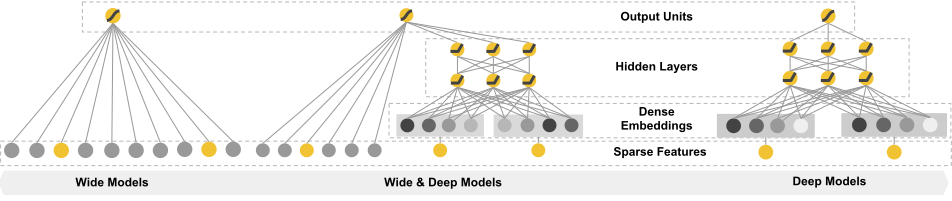
autoencoder = keras.Model(encoder_input, decoder_output, name = 'autoencoder')Combining Wide and Deep Models
The argument behind combining Wide and Deep models is to imitate human learning, i.e. by answering the question: can we teach computers to learn like humans do?
According to the premise hypothesis, human brains naturally combine memorization and generalization. Memorization refers to the ability to pattern-match inputs to outputs, e.g. hummingbirds fly, eagles fly, and so on. Generalization, on the other hand refers to the ability to identify a category of labels, for example, birds have wings (birds here, include hummingbirds, eagles, and so on).
“Combine the power of memorization and generalization on one unified machine learning model”
To accomplish a human imitating machine, Google has explored combining training of a wide linear model alongside a deep neural network. Google calls this process Wide & Deep Learning.
In practice:
- Deep: Stacking layers. Building a DNN.
- Wide: Dense embeddings, sparse features, leads to wider interpretations
For more information, see: https://ai.googleblog.com/2016/06/wide-deep-learning-better-together-with.html
For example implementation, refer to https://branyang.gitbooks.io/tfdocs/content/tutorials/wide_and_deep.html
Strength and weaknesses of Functional API
| Strengths | Explanation |
| Less Verbose | No super().__init__(...), No def call(self, ...):, |
| Model validation while defining its connectivity graph | Guarantees that any model you can build with the functional API will run. ll debugging — other than convergence-related debugging — happens statically during the model construction and not at execution time. This is similar to type checking in a compiler. |
| A functional model is plottable and inspectable | You can plot the model as a graph, and you can easily access intermediate nodes in this graph. |
| A functional model can be serialized or cloned | it is safely serializable and can be saved as a single file that allows you to recreate the exact same model without having access to any of the original code. |
| Weaknesses | Explanation |
| Doesn’t support Dynamic Architectures | The functional API treats models as DAGs of layers. This is true for most deep learning architectures, but not all — for example, recursive networks or Tree RNNs do not follow this assumption and cannot be implemented in the functional API. |
| Sometimes you have to write from scratch. | You have to make your own custom training or inference layers. |
Further reading
For more information about the functional API, see